The Ultimate Guide to Apache Spark 4.3

A release about time (mostly)

Spark 4.3.0 came out on October 30, including the more in depth Databricks release blog, which means my feeds are about to fill with listicles that paste the release notes into a numbered list and call it a day. I wanted to do something a little more in depth by reviewing each of the major features in this release as closely as possible, so that people can get a better idea of the expected behaviours and what it’s like to actually run the changes. Funnily, I expect a blog like this to have a shorter shelf life than usual as these releases are currently en track for a quarterly cadence, meaning Spark is about to get much more fully featured in the next year as it moves towards 5.0.

Reading the release notes end to end, I kept noticing that the big items all circle the same thing from different angles. Real-time Mode is about how quickly one record gets through a stateful query; SCD Type 2 is about how long a row’s history survives; ASOF JOIN is about which version of a fact was true at a given moment; and nanosecond timestamps are about how finely Spark can tell two moments apart in the first place. The remaining features (Project Feather, the Spark Connect observability work, DataFrame.zip, Python UDF transpilation) are about a different clock, which is yours: how long you wait between writing a query and seeing it run.

Most of Spark 4.3 is about time, both the data’s and yours: the scheduler learned to pipeline shuffles, so stateful streaming queries now run at millisecond latency; Auto CDC learned to keep history; SQL learned point-in-time joins and nanosecond precision; and the rest of the release shortens the loop between writing Spark code and finding out whether it works.

Every example here is a runnable script in spark-demos/demos/16_spark_43_guide, and every clip below is that script running against Spark 4.3.0 (pip install pyspark==4.3.0) on my machine. The Real-time Mode clips come from the Real-time Mode demo, which is a teaser for one of my upcoming Spark Streaming blog posts ;)

Below is a rundown of the new features and how to enable or take advantage of them.

Feature	Area	On by default?	How to turn it on
Stateful Real-time Mode	Structured Streaming	Yes (with the Real-time trigger)	.trigger(realTime="..."), update mode
SCD Type 2 in Auto CDC	Declarative Pipelines	Yes	STORED AS SCD TYPE 2 / stored_as_scd_type=2; target must support DSv2 row-level ops
Shuffle-free single-task execution	Project Feather	No	spark.sql.optimizer.singleTaskExecution.enabled=true
Arrow-native Dataset cache	Project Feather	No	spark.sql.cache.serializer=...ArrowCachedBatchSerializer (static)
Operation IDs, REST endpoints, with sessions	Spark Connect	Yes	nothing
Persistent local Connect server	Spark Connect	No	SPARK_LOCAL_CONNECT_REUSE=1
DataFrame.zip	PySpark, Connect	Yes	nothing
Python UDF transpilation	PySpark	No (experimental)	spark.sql.experimental.optimizer.transpilePyUDFs=true plus ANSI mode
ASOF JOIN	SQL	No (preview)	spark.sql.join.asofJoin.enabled=true
JSON_TABLE, VARIANT edit functions	SQL	Yes	nothing
Nanosecond timestamps	SQL	No (preview)	spark.sql.timestampNanosTypes.enabled=true
UNNEST, counter_diff, jaro_winkler_similarity	SQL	Yes	nothing
Reading inside tar, zip and 7z archives	File sources	No	spark.sql.files.archive.reader.enabled=true

Stateful Real-time Mode

Real-time Mode landed in 4.1 as a new trigger for Structured Streaming: instead of slicing a stream into micro-batches and waiting for each one to be planned, scheduled and committed, the query runs long-lived tasks that process records as they arrive and checkpoint on a much longer interval. The catch in 4.1 and 4.2 was that it only ran stateless queries (filters, projections, stream-static joins), because anything stateful needs a shuffle, and a classic shuffle is a blocking barrier where every map task has to finish writing before a single reduce task can read.

A new PipelinedShuffleDependency (SPARK-58185) routes data through a new StreamingShuffleManager (SPARK-57141), which pushes records to downstream tasks over Netty while the upstream tasks are still running. The DAGScheduler now schedules a pipelined group of stages together, fails them together, and refuses to start a group without enough task slots (SPARK-58263, SPARK-58398). This admission check prevents deadlock on a busy cluster: a consumer stage started without its producer would sit idle while holding cores. With that machinery in place, Real-time Mode supports streaming aggregation (SPARK-58635), dropDuplicates (SPARK-58508) and Scala/Java transformWithState (SPARK-57228), and is no longer marked @Experimental.

flowchart LR
    classDef old fill:#6b4a9b,fill-opacity:0.72,stroke:#6b4a9b,color:#ffffff
    classDef new fill:#c0661a,fill-opacity:0.72,stroke:#c0661a,color:#ffffff
    subgraph MB["Micro-batch: SortShuffleManager"]
        M1["map tasks<br/>write all output"]:::old --> W["shuffle files<br/>(barrier)"]:::old --> R1["reduce tasks<br/>start after"]:::old
    end
    subgraph RT["Real-time: StreamingShuffleManager"]
        M2["map tasks<br/>(long-running)"]:::new -->|"records pushed<br/>as they arrive"| R2["stateful tasks<br/>(running at the same time)"]:::new
    end

The query itself doesn’t change shape. In this deduplication and windowed-count step from the bookshop demo, only the trigger and output mode are specific to Real-time Mode:

trending = (clicks
    .withWatermark("ts", "10 seconds")
    .dropDuplicates(["event_id"])                       # resent clicks counted once
    .groupBy(F.window("ts", "10 seconds"), "aisle")
    .count())
 
(trending.writeStream.format("kafka")
    .outputMode("update")
    .trigger(realTime="30 seconds")                     # the whole change
    .start())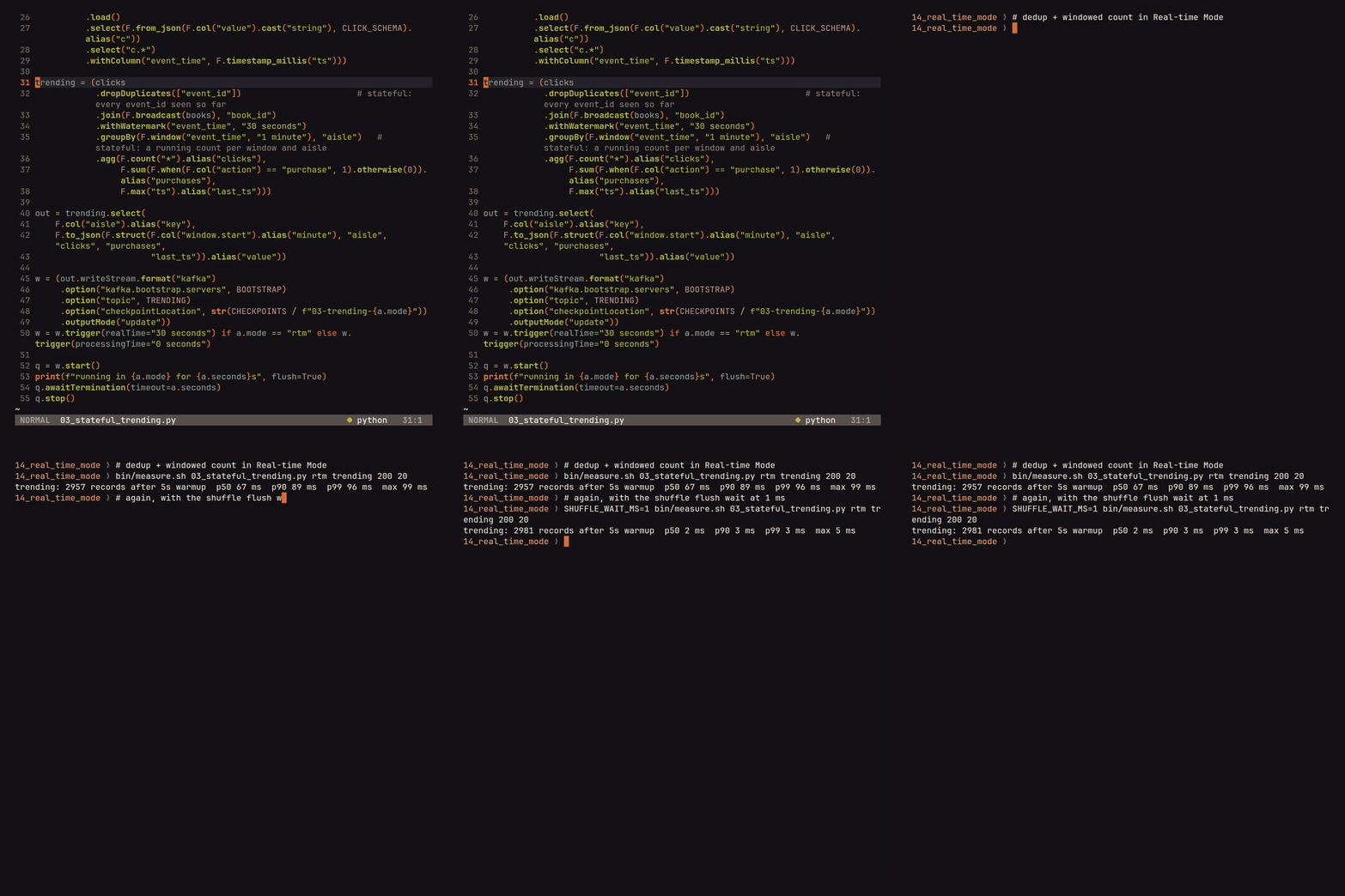

Measured end to end on my machine (from the click’s own timestamp to the broker’s append time on the output topic, 200 clicks a second for 45 seconds), the same query looks like this in each mode:

Step	Mode	p50 ms	p99 ms
Dedup + windowed count	micro-batch	237	645
Dedup + windowed count	Real-time	50	99
Dedup + windowed count	Real-time, flush wait 1 ms	2	41
transformWithState recommender	micro-batch	190	396
transformWithState recommender	Real-time	29	158

The 50 ms median comes from a timer. The streaming shuffle flushes when its buffer fills or spark.shuffle.streaming.networkBufferMaxWaitTimeMs expires; the default is 50 ms, and a lightly loaded query does not fill the buffer first. Reducing the wait to 1 ms brought the median down to 2 ms at the cost of more small network writes, a tradeoff to tune per workload rather than a useful global default. (The shorter run in the clip measured a 67 ms median and 96 ms p99 at the default, then 2 ms and 3 ms at 1 ms; the table contains the longer benchmark, and this amount of variation is normal for a single-machine test.) Databricks reports p99 latencies of 136 ms for dropDuplicates, 139 ms for a window aggregation and 141 ms for transformWithState on its benchmark workloads (SPARK-58884). Those results are not guarantees, and neither are mine, which come from one desktop with Kafka running in Docker.

For a stateful example, the recommender keeps a taste vector per shopper, built from book embeddings, in transformWithState and rescores the catalog on every click. The recommendations therefore change a few milliseconds after each click:

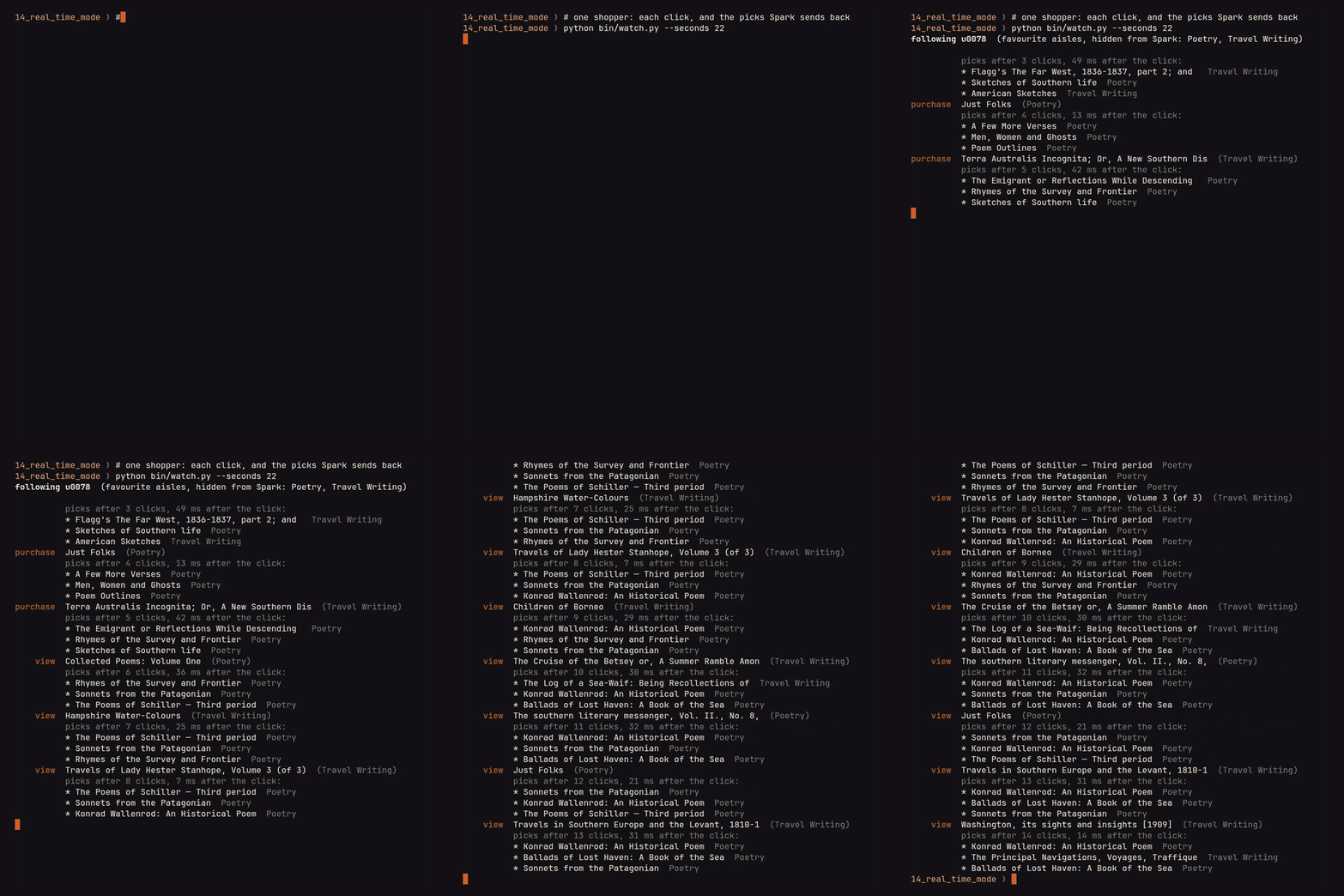
Real-time Mode still has several limits. transformWithState supports only Scala and Java, requires the RocksDB state store, and fires a processing-time timer on an idle key only when another row reaches its partition or the Real-time batch ends. ASOF JOIN is not supported. Pipelined stages also require cores concurrently, so the cluster must be sized for the whole pipeline rather than its widest stage.

SCD Type 2 in Auto CDC

Auto CDC arrived in 4.2 as the Declarative Pipelines way to turn a change feed into current state: give it keys, a sequencing column and a delete rule, and it keeps a target table in sync with MERGE, handling out-of-order and replayed events for you. In 4.2 that meant SCD Type 1, where the target only ever holds the latest version of each row. 4.3 adds SCD Type 2 (SPARK-58321), in Python (stored_as_scd_type=2, track_history_column_list), in SQL (STORED AS SCD TYPE 2, TRACK HISTORY ON) and through Spark Connect, so the target keeps every version, each bounded by __START_AT and __END_AT.

I reused the ghost kitchen from that post, this time tracking its menu. Each dish change arrives on a Kafka topic as a JSON event, as it would from a CDC tool. The pipeline has a Python source that reads the topic,

@dp.table
def menu_changes():
    return (spark.readStream.format("kafka")
        .option("kafka.bootstrap.servers", "localhost:29292")
        .option("subscribe", "menu-changes")
        .option("startingOffsets", "earliest")
        .load()
        .select(from_json(col("value").cast("string"), CHANGE).alias("e"))
        .select("e.*"))

and this one SQL statement:

-- Keep every version of every dish, not just the latest one.
CREATE STREAMING TABLE menu
FLOW AUTO CDC
FROM STREAM(menu_changes)
KEYS (dish_id)
SEQUENCE BY seq
APPLY AS DELETE WHEN op = 'DELETE'
COLUMNS * EXCEPT (op)
STORED AS SCD TYPE 2
TRACK HISTORY ON (price, station);

TRACK HISTORY ON controls which changes open a new version. Changes to unlisted columns update the current version in place, which prevents corrections such as typo fixes from creating history entries. Publishing change events in batches and running the pipeline after each batch shows both cases:

After the third run, the table contains the full history of each dish:

dish_id	dish	price	station	__START_AT	__END_AT
1	Birra tacos	14.00	grill	1	2
1	Birria tacos	14.00	plancha	2	NULL
2	Smash burger	13.50	grill	1	2
2	Smash burger	15.00	grill	2	NULL
3	Khao soi	16.00	wok	1	2

The typo fix at sequence 3 did not open a third row for the tacos because dish is not tracked; it updated the current version instead. Removing khao soi closed its window at sequence 2 rather than deleting it, preserving the previous menu state. __START_AT and __END_AT contain the sequencing value, which is an integer here but could instead be a commit timestamp.

As with Type 1, the target must support DSv2 row-level operations because Auto CDC applies each micro-batch with MERGE. Spark’s built-in file formats, including Parquet, fail at startup with AUTOCDC_TARGET_DOES_NOT_SUPPORT_MERGE; Apache Iceberg is the usual choice. Iceberg has not published a Spark 4.3 runtime yet (Maven Central currently stops at iceberg-spark-runtime-4.1), so I used an Iceberg runtime built from a branch with Spark 4.3 support. The Iceberg runtime, Kafka connector jars and spark.sql.extensions are static configurations and must be passed to spark-pipelines run, which accepts spark-submit arguments. Putting them in spark-pipeline.yml makes the CLI apply them to a live session and fail with CANNOT_MODIFY_CONFIG.

Project Feather: faster on small data

Spark has always been a slightly absurd tool for a 500-row file because its planning assumes the data is large: a groupBy gets a partial aggregate, a hash shuffle and a final aggregate, while an orderBy adds a range shuffle. Each exchange creates a stage boundary and another scheduling round trip. That overhead disappears into the work on a cluster; on a laptop, in a test suite, or in an agent running hundreds of small queries, it becomes the work. Project Feather (SPARK-56978) addresses that overhead, and 4.3 includes its first two pieces, both opt-in.

Shuffle-free single-task execution (SPARK-57851, spark.sql.optimizer.singleTaskExecution.enabled) notices when a query fragment reads something that fits in one partition (by default a single non-empty small file, or a local relation of up to 1,000 rows) and plans the scans, aggregations, distincts, windows, sorts and limits above it as one task with no exchanges at all. The same aggregation, with the flag off and then on:

def run(single_task, runs=20):
    spark.conf.set("spark.sql.optimizer.singleTaskExecution.enabled",
                   single_task)
    t = time.perf_counter()
    for _ in range(runs):
        # a fresh DataFrame each time, like a notebook cell or a test
        df = (spark.read.parquet(small)
              .groupBy("store").count().orderBy("store"))
        df.collect()
    return df, (time.perf_counter() - t) / runs * 1000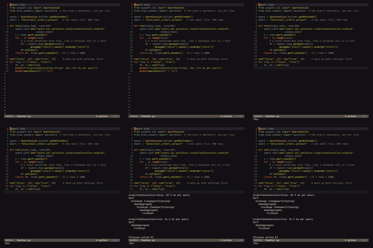

singleTaskExecution	Operators in the executed plan	Time per query
false	Sort, Exchange (range), HashAggregate, Exchange (hash), HashAggregate, FileScan	82.9 ms
true	Sort, HashAggregate, FileScan	51.2 ms

Both exchanges (and the shuffle query stages AQE wraps around them) are gone, and the query takes about 60% of the time, warm, on a session that’s already paid for JVM startup. The loop builds a new DataFrame every time on purpose, because that’s what a notebook cell, a test or an agent does. My first version collected the same DataFrame twenty times, and from the second collect on AQE reuses the shuffle output it already has, skipping the very stages Feather removes, so the two settings came out within a few milliseconds of each other. I wrote up the full benchmark (more queries, cold starts, and a test suite that went from 12.6 s to 5.2 s) in Benchmark Project Feather on a Fresh DataFrame.

The second piece is Arrow-native Dataset caching (SPARK-57268): set spark.sql.cache.serializer=org.apache.spark.sql.execution.columnar.ArrowCachedBatchSerializer when the application starts (it’s static) and df.cache() stores Arrow batches instead of Spark’s own columnar format, which pairs nicely with everything Arrow already does between the JVM and Python. Compression is available through spark.sql.execution.arrow.compression.codec, but it defaults to none, so out of the box the Arrow cache is bigger than the default one. Broader in-process local repartitioning was deferred to the next release (SPARK-57399).

Spark Connect: operation IDs and REST endpoints

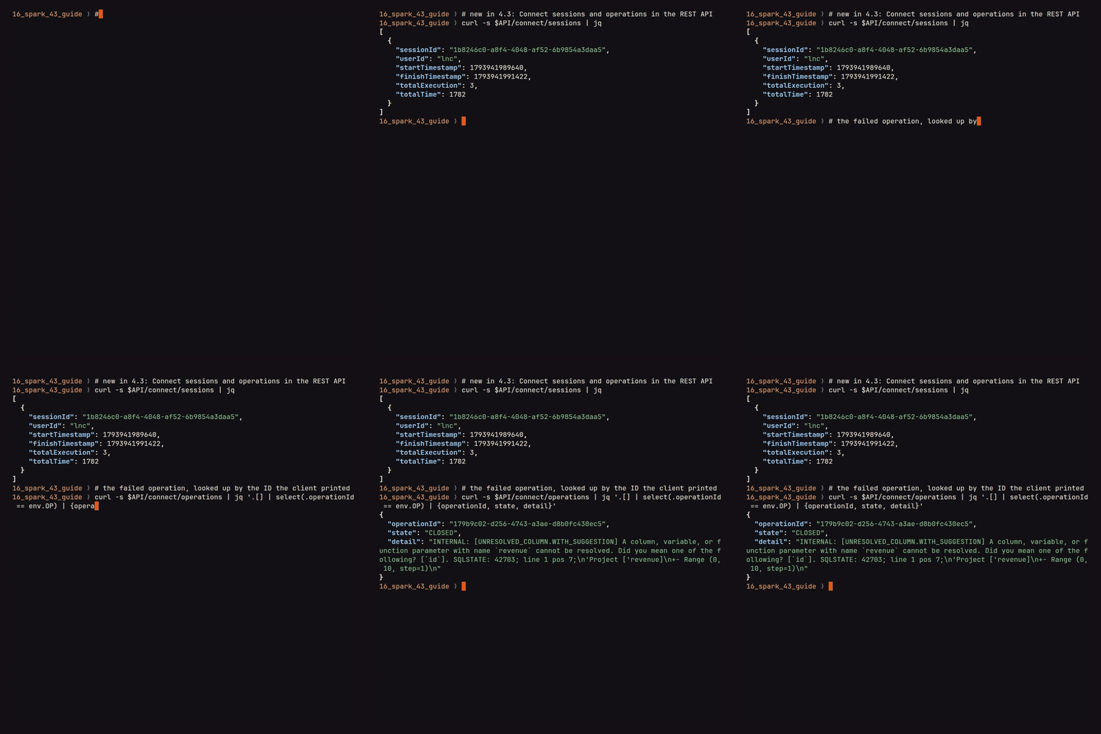
In my idiot’s guide to Connect I complained that debugging a Connect app means correlating a client-side error with a server you can’t see, and 4.3 fixes the two halves of that. First, the Python and Scala clients now generate an operation ID before every ExecutePlan request (SPARK-58547) and hand it back on success (df.executionInfo.operation_id) and, more usefully, on failure (e.operation_id on the exception), because a request that fails before its first response never learned a server-generated ID. The server publishes the same ID as a Spark local property, so listeners and executor tasks can see it too.

remote = SparkSession.builder.remote("sc://localhost:15043")
with remote.getOrCreate() as spark:      # new in 4.3: sessions are context managers
    ok = spark.sql("SELECT count(*) AS n FROM range(1000000)")
    ok.collect()
    print("succeeded, operation", ok.executionInfo.operation_id)
 
    try:
        spark.sql("SELECT revenue FROM range(10)").collect()
    except Exception as e:   # the client knows the ID even on failure
        print("failed,    operation", e.operation_id)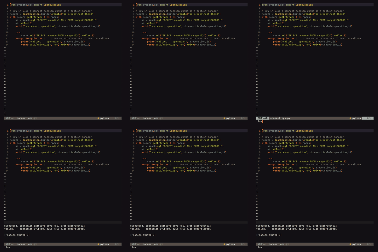

Second, the server’s sessions and operations are now in the monitoring REST API (SPARK-57941), next to the SQL and streaming endpoints, where before they only lived in the Connect tab of the UI:

curl -s $API/connect/sessions | jq
curl -s $API/connect/operations | jq '.[] | select(.operationId == env.OP)'

Take the ID the client printed for the failure, and the server’s record of that same operation has its state, timings, the SQL execution it ran and the full error:

Because the Connect listener writes these events to the event log, the same endpoints work in the History Server after the application exits. Other Connect changes include the session context manager above (SPARK-58159), a SQLContext wrapper for existing code (SPARK-57021), an experimental SPARK_LOCAL_CONNECT_REUSE=1 setting that keeps a local Connect server alive between runs (SPARK-57787), and broader support in the Connect JDBC driver for complex types, DatabaseMetaData keys and SQLSTATE class 08 connection errors. The INVALID_HANDLE.SESSION_* errors changed SQLSTATE from HY000 to 08003, so retry logic that matches SQLSTATE may need updating. Connect Gateway and the Rust-backed Python client are concurrent projects, not Spark 4.3 features.

PySpark: DataFrame.zip and UDF transpilation

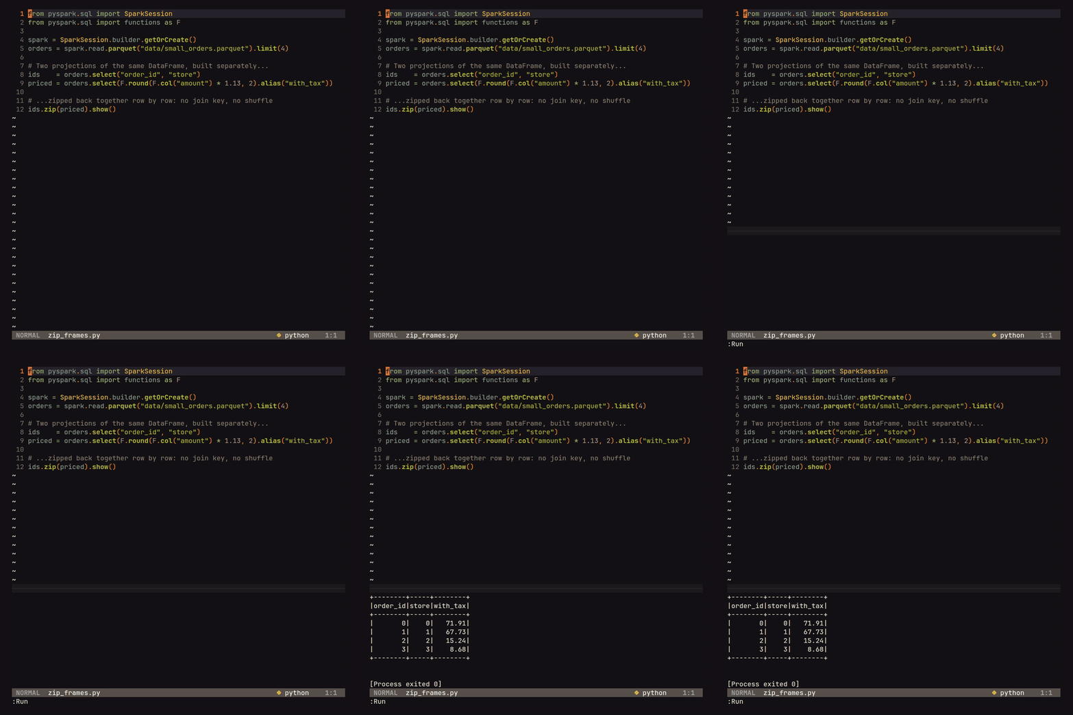
DataFrame.zip (SPARK-55886, with Connect support in SPARK-57247) places two column projections of the same DataFrame side by side, row for row, without a join key. It replaces joins built on monotonically_increasing_id(), whose rows are not guaranteed to align. Both sides must originate from the same plan, with matching filters, sorts, joins and aggregations beneath the projections.

The experimental Python UDF transpiler (SPARK-55206) is the one I’ve been waiting for since the UDF showdown, where the conclusion was that the fastest Python UDF is the one that never runs Python. With spark.sql.experimental.optimizer.transpilePyUDFs=true and ANSI mode on, PySpark reads simple UDF bodies when you define them and lowers them to Catalyst expressions, so len(dish) becomes Spark’s own length and the BatchEvalPython step (and the Python worker, and the serialization) drops out of the plan:

spark = (SparkSession.builder
         .config("spark.sql.ansi.enabled", "true")  # transpiling needs ANSI
         .getOrCreate())
 
@udf("int", useArrow=False)
def name_length(dish: str) -> int:
    return len(dish)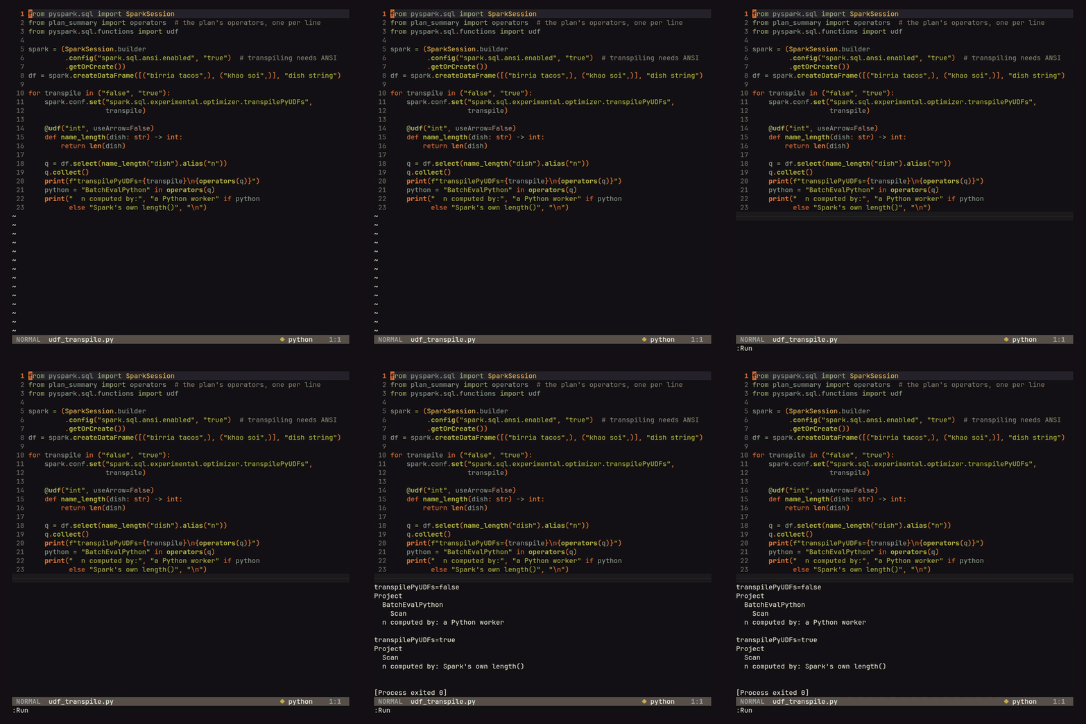

The restrictions are not all documented together, so I read pyspark/sql/udf.py to collect them. Transpilation applies only to non-Arrow batched UDFs (hence useArrow=False), classic PySpark, ANSI mode, and function bodies that PySpark can recover from source, excluding an inline lambda passed directly to udf(). With ANSI mode disabled, PySpark warns and falls back because the generated expressions use ANSI semantics. The transpiler also preserves Python behavior where Spark differs: a transpiled len raises on NULL as CPython would, represented in the full plan by a raise_error branch. Parameter type hints keep the generated plan small. Other PySpark changes bound UDF input batches by bytes, implement more pandas API on Spark functions natively, remove Python 3.10 support, and raise the minimum NumPy version to 1.23.2.

Spark SQL: ASOF JOIN, JSON_TABLE, VARIANT edits and nanoseconds

ASOF JOIN (SPARK-58092) is the point-in-time join: for each row on the left, the single closest row on the right that satisfies a MATCH_CONDITION comparison, optionally within an equality ON or USING key. In my Rust client post I had to pull a Spark result into DuckDB to do exactly this, so it’s nice to have it native, with a dedicated sort-merge operator. The canonical ML case is matching each prediction to the feature version that had actually been published when the prediction was made:

SELECT p.made_at, p.score, f.version AS features_used, f.published_at
FROM predictions p
ASOF JOIN feature_versions f
MATCH_CONDITION (p.made_at >= f.published_at)  -- latest one out by then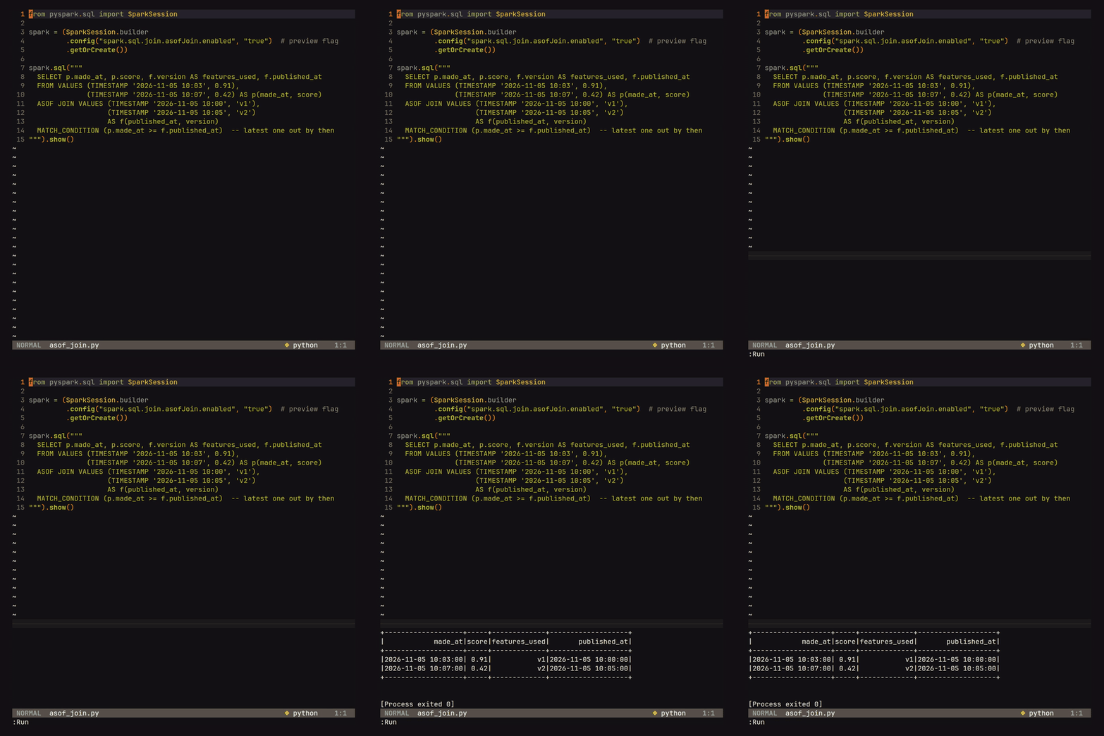

The 10:03 prediction gets v1 from 10:00 and never v2 from 10:05, which didn’t exist yet (using it would be leakage), and the 10:07 prediction gets v2 alone, where a plain >= join would return both versions and leave you to pick the latest yourself, which is exactly where the leakage bugs usually creep in. It’s a preview: spark.sql.join.asofJoin.enabled is off by default (and internal, so it won’t show up in SET -v), only INNER and LEFT OUTER are supported, and in streaming only stream-static works, with the stream on the left.

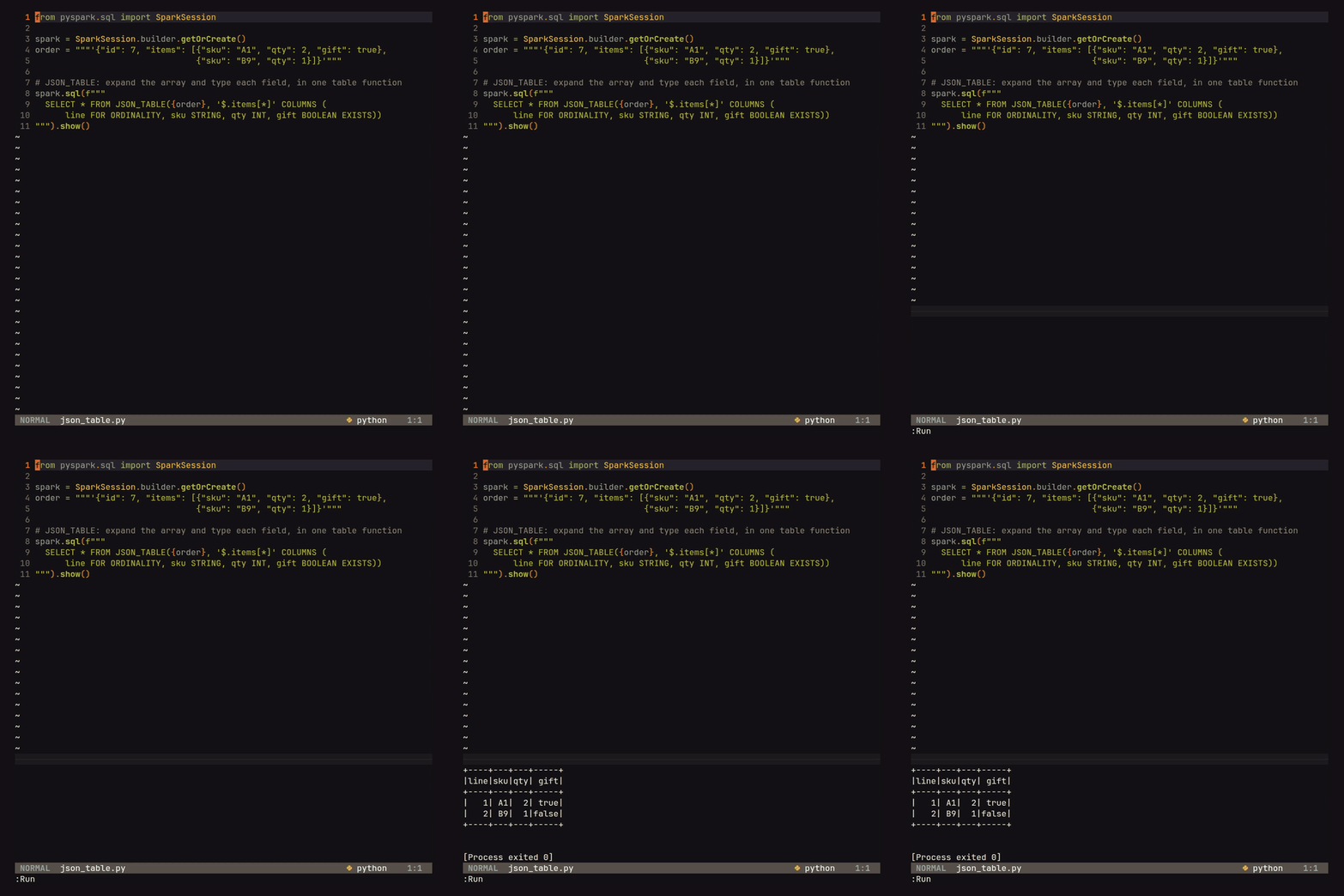
JSON_TABLE (SPARK-58366) is the SQL-standard table function for expanding a JSON array into typed rows. It also supports FOR ORDINALITY and EXISTS columns:

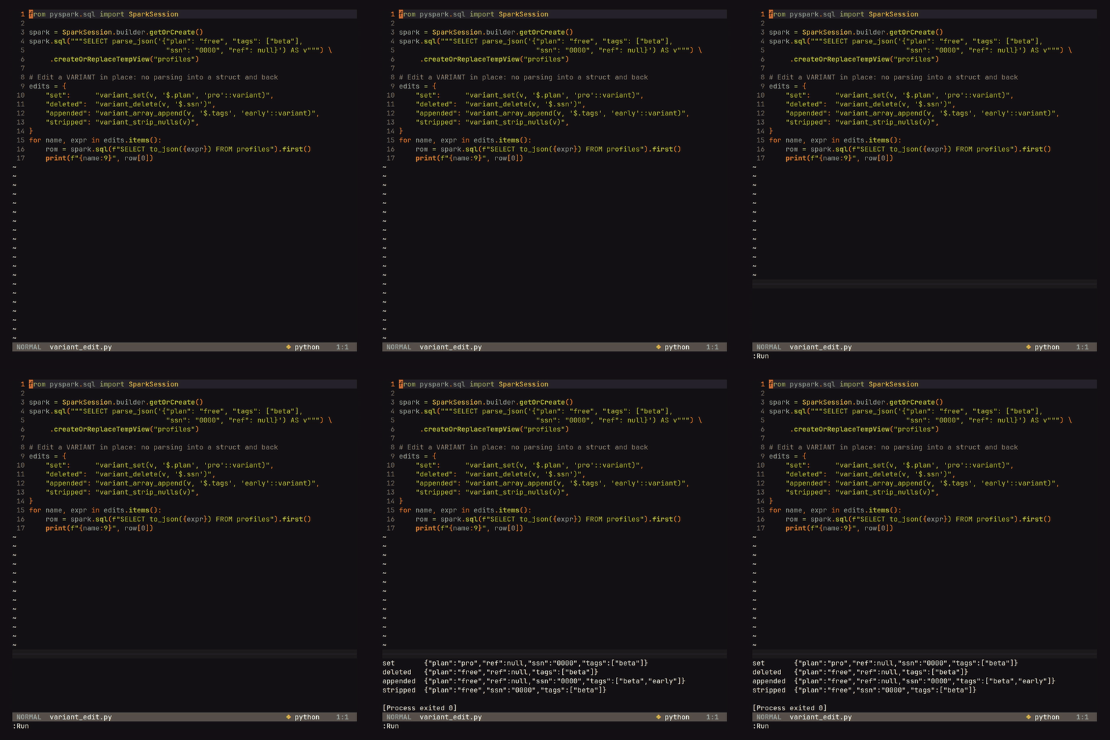
And VARIANT values can finally be edited in place with variant_set, variant_insert, variant_delete, variant_array_append and variant_strip_nulls (plus try_ versions), instead of being parsed into a struct and serialized back:

Nanosecond timestamps (SPARK-56876) add TIMESTAMP_NTZ(p) and TIMESTAMP_LTZ(p) for precisions 7 to 9, with unix_nanos, timestamp_nanos, current_timestamp(p), datetime functions, interval arithmetic, and Parquet, ORC, JSON, CSV, Avro, JDBC, Arrow and Connect support. Spark’s TIMESTAMP has been microseconds since forever, which means two market events a nanosecond apart (or two rows from a Parquet file written by something that does use nanoseconds) silently became the same instant:

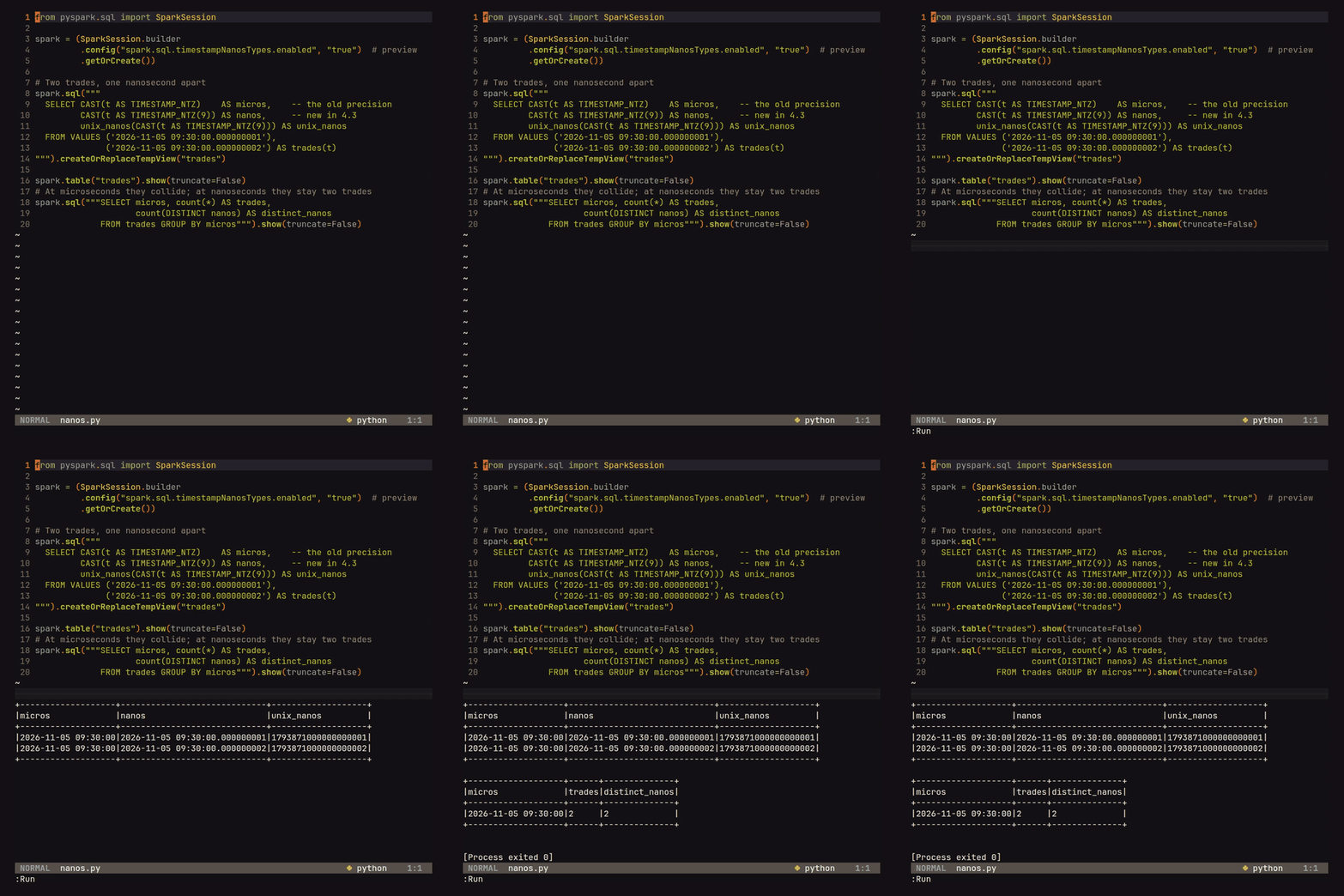
Nanosecond timestamps remain a preview behind spark.sql.timestampNanosTypes.enabled, and the Databricks release post warns that they may change incompatibly. Typed literals such as TIMESTAMP_NTZ(9) '...' do not parse yet, so values must be cast from strings. I would not use the type for production work yet: while building this demo, I found a query that returns an incorrect count when a nanosecond column appears beside other DISTINCT aggregates in the same SELECT; I am reducing the reproduction before filing it. The TIME type also gained nanosecond precision and broader connector support, but remains disabled behind an internal flag.

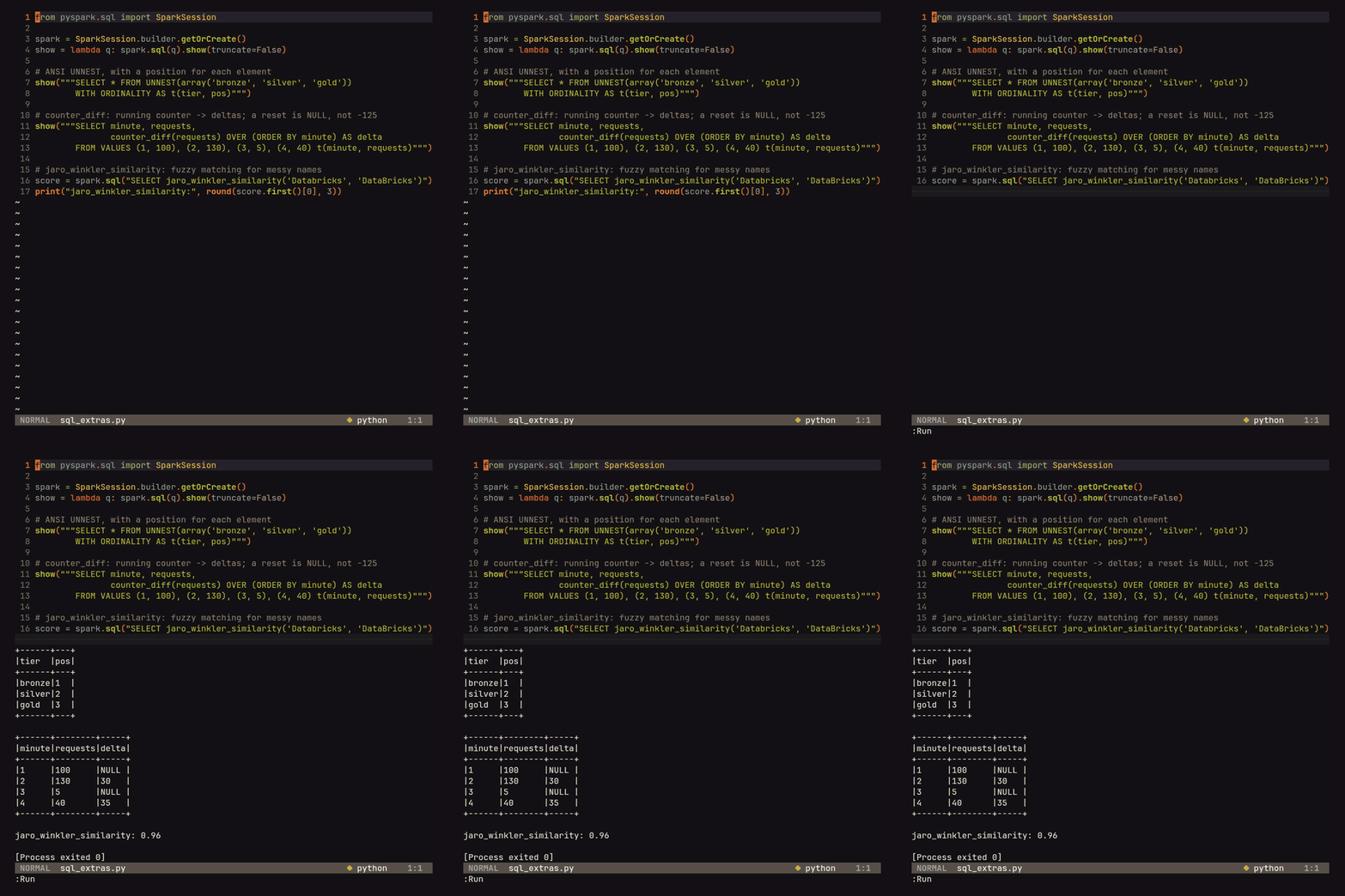
Other SQL additions include ANSI UNNEST in FROM, with WITH ORDINALITY; counter_diff, a window function that converts a running counter such as requests served or bytes sent into per-interval deltas and returns NULL after a reset; and jaro_winkler_similarity for fuzzy name matching:

Also new and not filmed: @-syntax time travel on table names (t@v3, or t@20261105093000000 in the fixed 17-digit yyyyMMddHHmmssSSS form), COMMENT ON COLUMN, dynamic table options on UPDATE, MERGE and DELETE, AS JSON output for SHOW TABLES and SHOW PARTITIONS, collect_union, to_base32/from_base32, and a BIN BY relation operator behind a flag.

Reading files inside archives

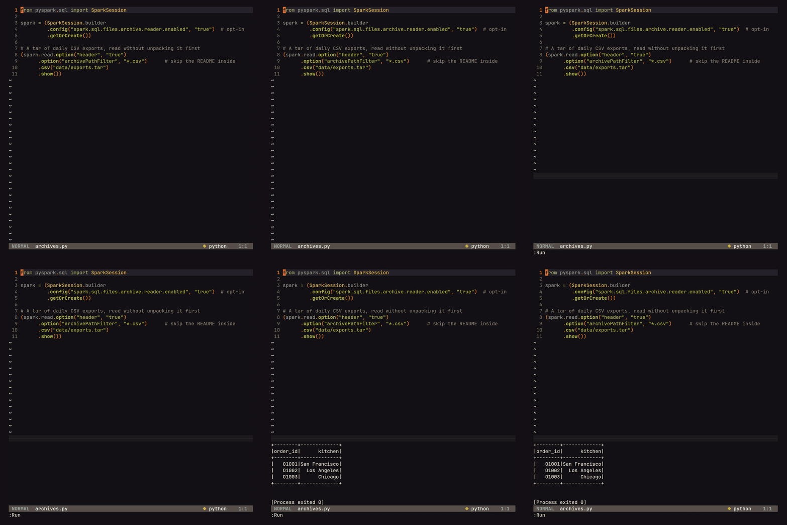
The archive reader may be the feature I use most. With spark.sql.files.archive.reader.enabled=true, file sources read entries inside tar, zip and 7z archives as separate files, including during schema inference; archivePathFilter selects the entries to read. This removes the usual step of unpacking a vendor’s nightly archive into a temporary directory:

Other changes in Spark 4.3

A lot of 4.3 is engine work you get for free. ReplaceHashWithSortAgg and combining adjacent partial and final aggregates are now on by default, whole-stage codegen covers UNION, AQE can convert a sort-merge join to a shuffled hash join in the physical plan, nested column pruning reaches into transform over arrays of structs, and the vectorized Parquet reader got faster decoding paths and a BYTE_STREAM_SPLIT reader. There’s an opt-in to spread NULL outer join keys across partitions (a classic skew source), fractional spark.task.cpus, spark.rdd.compress on by default, and the Spark UI’s Content Security Policy on by default. On Kubernetes the official images move to Ubuntu 26.04 with Python 3.14, and containers drop allowPrivilegeEscalation by default.

A few changes can change results or break things on upgrade, all in the migration guide: exact percentile/median may differ in the last ULP; Dataset.observe metrics now count only the last successful task attempt; HAVING is applied before window functions when the SELECT also has a generator (fixing wrong results); non-deterministic filters are no longer pushed to DSv2 sources; Thrift Server sessions can no longer set JVM system properties; and the AQE rule DynamicJoinSelection was renamed DemoteBroadcastHashJoin, so an exclusion by the old name now silently does nothing.

In Summary

• Stateful Real-time Mode: pipelined shuffles let dedup, aggregation and transformWithState (Scala/Java) run at millisecond latency with only a trigger change, and the default median is a 50 ms flush timer you can tune.
• SCD Type 2 in Auto CDC keeps every version with __START_AT/__END_AT; TRACK HISTORY ON decides what opens a new version, and the target needs a row-level-capable catalog like Iceberg (whose 4.3 runtime isn’t published yet).
• Project Feather is opt-in: single-task execution removes the exchanges from small queries (about 1.6x faster here, warm), and the Arrow cache serializer is a static config.
• Spark Connect gives you an operation ID on success and failure, and the same operation in the server’s REST API.
• DataFrame.zip replaces the monotonically_increasing_id join hack; UDF transpilation removes Python from simple UDFs if you’re on classic PySpark with ANSI on.
• ASOF JOIN, nanosecond timestamps and archive reading are all behind flags; JSON_TABLE, VARIANT edits, UNNEST and counter_diff just work.

Most of it comes back to time: a record’s few milliseconds through a stateful query, a dish’s price history that never gets overwritten, the feature version that was true at 10:03, the nanosecond between two trades, and the milliseconds a small query no longer spends on shuffles. On a quarterly cadence, expect all of it to keep moving faster than it used to.

Further reading

• Introducing Apache Spark 4.3, the Databricks launch post, with the Real-time Mode benchmarks.
• Spark 4.3.0 release notes, every change with its JIRA.
• SQL migration guide, 4.2 to 4.3, for the behaviour changes above.
• spark-demos/demos/16_spark_43_guide, every script in this post, plus the film scripts.
• AUTO CDC: Turning an event log into current state, the SCD Type 1 post this builds on.